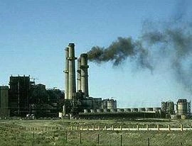
Air pollution dispersion modeling

Crude oil-fired power plant — Industrial air pollution source

Atmospheric dispersion modeling is the mathematical simulation of how air pollutants disperse in the ambient atmosphere. It is performed with computer programs that solve the mathematical equations and algorithms which simulate the pollutant dispersion. The dispersion models are used to estimate or to predict the downwind concentration of air pollutants emitted from sources such as industrial plants, vehicular traffic or accidental chemical releases.

Such models are important to governmental agencies tasked with protecting and managing the ambient air quality. The models are typically employed to determine whether existing or proposed new industrial facilities are or will be in compliance with the National Ambient Air Quality Standards (NAAQS) in the United States or similar regulations in other nations. The models also serve to assist in the design of effective control strategies to reduce emissions of harmful air pollutants. During the late 1960's, the Air Pollution Control Office of the U.S. Environmental Protection Agency (U.S. EPA) initiated research projects to develop models for use by urban and transportation planners.^[1]

Air dispersion models are also used by emergency management personnel to develop emergency plans for accidental chemical releases. The results of dispersion modeling, using worst case accidental releases and meteorological conditions, can provide estimated locations of impacted areas and be used to determine appropriate protective actions. At industrial facilities in the United States, this type of consequence assessment or emergency planning is required under the Clean Air Act (CAA) codified in Part 68 of Title 40 of the Code of Federal Regulations.

The dispersion models vary depending on the mathematics used to develop the model, but all require the input of data that may include:

Meteorological conditions such as wind speed and direction, the amount of atmospheric turbulence (as characterized by what is called the "stability class"), the ambient air temperature, the height to the bottom of any inversion aloft that may be present, cloud cover and solar radiation.
The emission parameters such the type of source (i.e., point, line or area), the mass flow rate, the source location and height, the source exit velocity, and the source exit temperature.
Terrain elevations at the source location and at receptor locations, such as nearby homes, schools, businesses and hospitals.
The location, height and width of any obstructions (such as buildings or other structures) in the path of the emitted gaseous plume as well as the terrain surface roughness (which may be characterized by the more generic parameters "rural" or "city" terrain).

Many of the modern, advanced dispersion modeling programs include a pre-processor module for the input of meteorological and other data, and many also include a post-processor module for graphing the output data and/or plotting the area impacted by the air pollutants on maps. The plots of areas impacted usually include isopleths showing areas of pollutant concentrations that define areas of the highest health risk. The isopleths plots are useful in determining protective actions for the public and first responders.

The atmospheric dispersion models are also known as atmospheric diffusion models, air dispersion models, air quality models, and air pollution dispersion models.

Atmospheric layers

Discussion of the layers in the Earth's atmosphere is needed to understand where airborne pollutants disperse in the atmosphere. The layer closest to the Earth's surface is known as the troposphere. It extends from sea-level up to a height of about 18 km and contains about 80 percent of the mass of the overall atmosphere. The stratosphere is the next layer and extends from 18 km up to about 50 km. The third layer is the mesosphere which extends from 50 km up to about 80 km. There are other layers above 80 km, but they are insignificant with respect to atmospheric dispersion modeling.

The lowest part of the troposphere is called the atmospheric boundary layer (ABL) or the planetary boundary layer (PBL) and extends from the Earth's surface up to about 1.5 to 2.0 km in height. The air temperature of the atmospheric boundary layer decreases with increasing altitude until it reaches what is called the inversion layer (where the temperature increases with increasing altitude) that caps the atmospheric boundary layer. The upper part of the troposphere (i.e., above the inversion layer) is called the free troposphere and it extends up to the 18 km height of the troposphere.

The ABL is the most important layer with respect to the emission, transport and dispersion of airborne pollutants. The part of the ABL between the Earth's surface and the bottom of the inversion layer is known as the mixing layer. Almost all of the airborne pollutants emitted into the ambient atmosphere are transported and dispersed within the mixing layer. Some of the emissions penetrate the inversion layer and enter the free troposphere above the ABL.

In summary, the layers of the Earth's atmosphere from the surface of the ground upwards are: the ABL made up of the mixing layer capped by the inversion layer; the free troposphere; the stratosphere; the mesosphere and others. Many atmospheric dispersion models are referred to as boundary layer models because they mainly model air pollutant dispersion within the ABL. To avoid confusion, models referred to as mesoscale models have dispersion modeling capabilities that can extend horizontally as much as a few hundred kilometres. It does not mean that they model dispersion in the mesosphere.

Gaussian air pollutant dispersion equation

The technical literature on air pollution dispersion is quite extensive and dates back to the 1930s and earlier. One of the early air pollutant plume dispersion equations was derived by Bosanquet and Pearson.^[2] Their equation did not assume Gaussian distribution nor did it include the effect of ground reflection of the pollutant plume.

Sir Graham Sutton derived an air pollutant plume dispersion equation in 1947^[3][4] which did include the assumption of Gaussian distribution for the vertical and crosswind dispersion of the plume and also included the effect of ground reflection of the plume.

Under the stimulus provided by the advent of stringent environmental control regulations, there was an immense growth in the use of air pollutant plume dispersion calculations between the late 1960s and today. A great many computer programs for calculating the dispersion of air pollutant emissions were developed during that period of time and they were commonly called "air dispersion models". The basis for most of those models was the Complete Equation For Gaussian Dispersion Modeling Of Continuous, Buoyant Air Pollution Plumes shown below:^[5][6]

$C = \frac{\;Q}{u}\cdot\frac{\;f}{\sigma_y\sqrt{2\pi}}\;\cdot\frac{\;g_1 + g_2 + g_3}{\sigma_z\sqrt{2\pi}}$

where:
$f$	= crosswind dispersion parameter
	= $\exp \;[-\,y^{2}/\,(2\;\sigma _{y}^{2}\;)\;]$
$g$	= vertical dispersion parameter = $\,g_{1}+g_{2}+g_{3}$
$g_1$	= vertical dispersion with no reflections
	= $\;\exp \;[-\,(z-H)^{2}/\,(2\;\sigma _{z}^{2}\;)\;]$
$g_{2}$	= vertical dispersion for reflection from the ground
	= $\;\exp \;[-\,(z+H)^{2}/\,(2\;\sigma _{z}^{2}\;)\;]$
$g_3$	= vertical dispersion for reflection from an inversion aloft
	= $\sum _{m=1}^{\infty }\;{\big \{}\exp \;[-\,(z-H-2mL)^{2}/\,(2\;\sigma _{z}^{2}\;)\;]$
	$+\,\exp \;[-\,(z+H+2mL)^{2}/\,(2\;\sigma _{z}^{2}\;)\;]$
	$+\,\exp \;[-\,(z+H-2mL)^{2}/\,(2\;\sigma _{z}^{2}\;)\;]$
	$+\,\exp \;[-\,(z-H+2mL)^{2}/\,(2\;\sigma _{z}^{2}\;)\;]{\big \}}$
$C$	= concentration of emissions, in g/m³, at any receptor located:
	x meters downwind from the emission source point
	y meters crosswind from the emission plume centerline
	z meters above ground level
$Q$	= source pollutant emission rate, in g/s
$u$	= horizontal wind velocity along the plume centerline, m/s
$H$	= height of emission plume centerline above ground level, in m
$\sigma_z$	= vertical standard deviation of the emission distribution, in m
$\sigma_y$	= horizontal standard deviation of the emission distribution, in m
$L$	= height from ground level to bottom of the inversion aloft, in m
$\exp$	= the exponential function

The above equation not only includes upward reflection from the ground, it also includes downward reflection from the bottom of any inversion lid present in the atmosphere.

The sum of the four exponential terms in $g_3$ converges to a final value quite rapidly. For most cases, the summation of the series with m = 1, m = 2 and m = 3 will provide an adequate solution.

$\sigma_z$ and $\sigma_y$ are functions of the atmospheric stability class (i.e., a measure of the turbulence in the ambient atmosphere) and of the downwind distance to the receptor. The two most important variables affecting the degree of pollutant emission dispersion obtained are the height of the emission source point and the degree of atmospheric turbulence. The more turbulence, the better the degree of dispersion.

Whereas older models rely on stability classes for the determination of $\sigma_y$ and $\sigma_z$ , more recent models increasingly rely on Monin-Obukhov similarity theory to derive these parameters.

Briggs plume rise equations

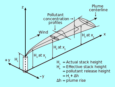
The Gaussian air pollutant dispersion equation (discussed above) requires the input of H which is the pollutant plume's centerline height above ground level. H is the sum of H_s (the actual physical height of the pollutant plume's emission source point) plus ΔH (the plume rise due the plume's buoyancy).

Gaussian Plume — Diagram of a buoyant Gaussian pollution plume

To determine ΔH, many if not most of the air dispersion models developed between the late 1960s and the early 2000s used what are known as "the Briggs equations." G.A. Briggs first published his plume rise observations and comparisons in 1965.^[7] In 1968, at a symposium sponsored by CONCAWE (a Dutch organization), he compared many of the plume rise models then available in the literature.^[8] In that same year, Briggs also wrote the section of the publication edited by Slade^[9] dealing with the comparative analyses of plume rise models. That was followed in 1969 by his classical critical review of the entire plume rise literature,^[10] in which he proposed a set of plume rise equations which have become widely known as "the Briggs equations". Subsequently, Briggs modified his 1969 plume rise equations in 1971 and in 1972.^[11][12]

Briggs divided air pollution plumes into these four general categories:

Cold jet plumes in calm ambient air conditions
Cold jet plumes in windy ambient air conditions
Hot, buoyant plumes in calm ambient air conditions
Hot, buoyant plumes in windy ambient air conditions

Briggs considered the trajectory of cold jet plumes to be dominated by their initial velocity momentum, and the trajectory of hot, buoyant plumes to be dominated by their buoyant momentum to the extent that their initial velocity momentum was relatively unimportant. Although Briggs proposed plume rise equations for each of the above plume categories, it is important to emphasize that "the Briggs equations" which become widely used are those that he proposed for bent-over, hot buoyant plumes.

In general, the Briggs equations for bent-over, hot buoyant plumes are based on observations and data involving plumes from typical combustion sources such as the flue gas stacks from steam-generating boilers burning fossil fuels in large power plants. Therefore the stack exit velocities were probably in the range of 20 to 100 ft/s (6 to 30 m/s) with exit temperatures ranging from 250 to 500 °F (120 to 260 °C).

A logic diagram for using the Briggs equations^[5] to obtain the plume rise trajectory of bent-over buoyant plumes is presented below:

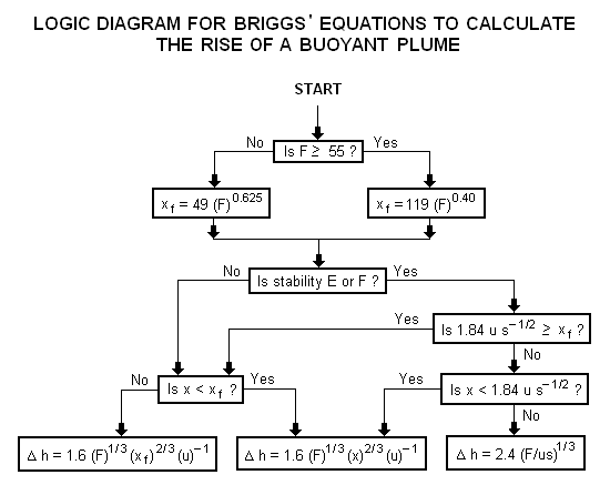
where:
Δh	= plume rise, in m
F	= buoyancy factor, in m⁴s⁻³
x	= downwind distance from plume source, in m
x_f	= downwind distance from plume source to point of maximum plume rise, in m
u	= windspeed at actual stack height, in m/s
s	= stability parameter, in s⁻²

The above parameters used in the Briggs equations are discussed in Beychok's book.^[5]

References

[1] J.C. Fensterstock et al, "Reduction of air pollution potential through environmental planning", JAPCA, Vol. 21,
   No. 7, 1971.
[2] C.H. Bosanquet and J.L. Pearson, "The spread of smoke and gases from chimneys", Trans. Faraday Soc.,
   32:1249, 1936.
[3] O.G. Sutton, "The problem of diffusion in the lower atmosphere", QJRMS, 73:257, 1947.
[4] O.G. Sutton, "The theoretical distribution of airborne pollution from factory chimneys", QJRMS, 73:426, 1947.
[5] M.R. Beychok (2005), Fundamentals Of Stack Gas Dispersion, 4th Edition, self-published, ISBN 0-9644588-0-2.
[6] D. B. Turner (1994),Workbook of atmospheric dispersion estimates: an introduction to dispersion modeling, 2nd
   Edition, CRC Press, ISBN 1-56670-023-X.
[7] G.A. Briggs, "A plume rise model compared with observations", JAPCA, 15:433–438, 1965.
[8] G.A. Briggs, "CONCAWE meeting: discussion of the comparative consequences of different plume rise
   formulas", Atmos. Envir., 2:228–232, 1968.
[9] D.H. Slade (editor), "Meteorology and atomic energy 1968", Air Resources Laboratory, U.S. Dept. of Commerce,
   1968.
[10] G.A. Briggs, "Plume Rise", USAEC Critical Review Series, 1969.
[11] G.A. Briggs, "Some recent analyses of plume rise observation", Proc. Second Internat'l. Clean Air Congress,
  Academic Press, New York, 1971.
[12] G.A. Briggs, "Discussion: chimney plumes in neutral and stable surroundings", Atmos. Envir., 6:507–510,
  1972.

Air pollution dispersion modeling

Contents

Atmospheric layers

Gaussian air pollutant dispersion equation

Briggs plume rise equations

References

Further reading

Fan Feed